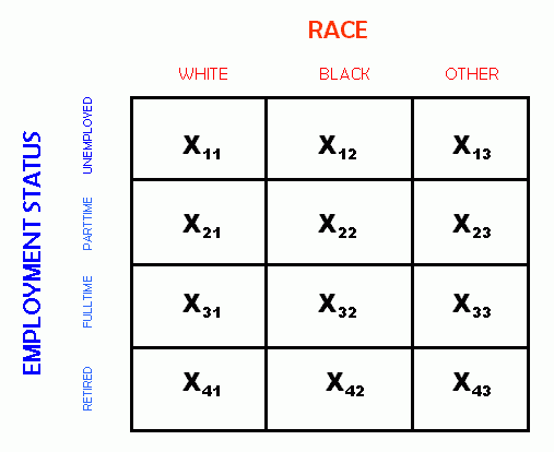
To perform the Chi-square calculation, first one must construct a table called a "cross-tabulation" or "cross-tab" or "X-tab".
In this tutorial you will examine the following concepts:
A crosstabulation table has a row for each category of one variable, and a column for each category of the other variable. It makes no difference which of the two variables is used for the rows and which for the columns.
The table has three kinds of scores. One kind is the cell entry scores, which store the number of cases in any "box" in a table. That is, a cell entry score is the number of cases with a specific value for each variable, such as whites who work full time. In the crosstabulation table below, variables such as X11 and X23 are used to denote the number of cases in a given cell

The second type of score is called a marginal total or "marginal" value. The marginals are each a summation across a particular row or column. In our example, the marginals indicate the total number of unemployed people, the total number of people employed parttime, the total number of people employed fulltime, the total number of people who are retired, the total number of white people, the total number of black people, and the total number of people of other races. Note that knowing the total number of black people tells us nothing about the relationship (if any) between blacks and level of employment.
The third type of score is the grand total for all of the cases in the entire table.
In the following picture, the marginals and the grand total have been added to the table.
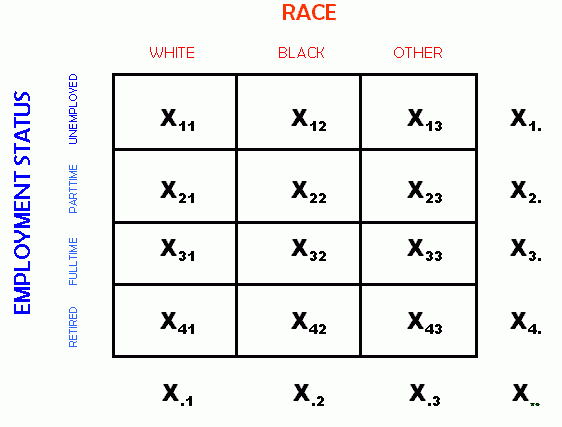
In the table above, the variable X1. denotes the total for row 1. Note the dot in the variable subscript in the second position of the subscript -- this indicates that the variable is a row marginal. In similar fashion the column 1 marginal is denoted by X.1. Finally, the grand total is denoted by X...
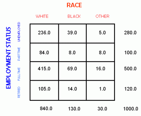
In a bivariate crosstabulation we are measuring the relationship between the "expected" and "observed" counts for the categories of two variables. Below is a cross tablulation table, with the total number of cases for each category shown in the marginals.
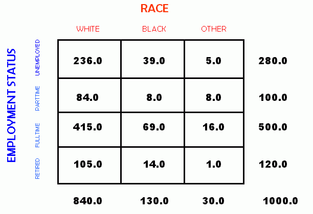
To use crosstabulation, we must build two matrices. We must construct one for the expected number of occurences in each cell, and another for the observed number of occurences in each cell.
As a practical matter, a researcher with a data set to analyze will typically begin with the marginals and total already available. The initial step to analysis is then to fill in the cell values. If we know the marginals, we need know only two observed cell counts in a given row of a 4 x 3 table to be able to calculate the count for the last cell in that row. Likewise, if we know three of the cell values in a column along with the marginal, we can compute the last cell value. Thus, we can fill in the following table from the information provided. As an example, see the table below and the activity which follows.
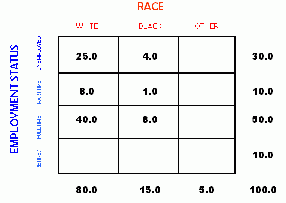
Activity 1
Before we can determine whether there is a relationship between race and employment level, we must first determine the "expected" result if there is no such relationship -- that is, if race does not affect the probability of having fulltime employment. Note that the claim "There is no relationship between race and employment level" is the Null Hypothesis for this question.
The expected frequency f(XRC) for any cell XRC is calculated as E(XRC) = (RC)/T where R is the row total, C is the column total, and T is the grand total for the table.
Think about the logic of this calculation. C/T represents the fraction of the grand total in a given column. The cases in any given column are divided among the cells of that column. The formula for E(XRC) tells us how the cases for a given column would be distributed among the cells if there was no relationship between the variables. For example, if Row 1 of the table has twice as many cases as Row 2, then the Column 1, Row 1 cell can be expected to have twice as many cases as the Column 1, Row 2 cell, if only random chance is operating.
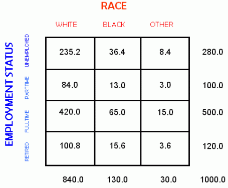
For our example, computing the expected table would be as follows:
4 x 3 Table for Computation of "Expected" Race and Employment Status
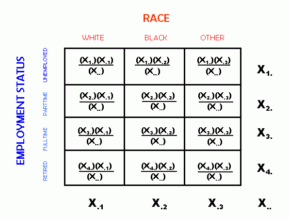
When answering the following questions, refer to the above diagrams for assistance.
Activity 2
| OBSERVED FREQUENCIES | EXPECTED FREQUENCIES |
 |
 |
The difference between observed and expected scores is then seen in the following 4 x 3 table:
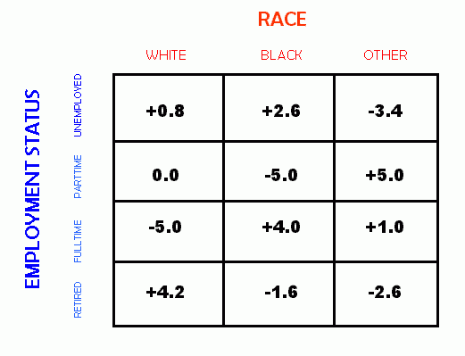
We now have the necessary information to calculate Chi-square for these
two variables.
The formula for Chi-square is:  where
where  is the observed frequency
for a given cell and
  is the
expected frequency for that same cell, and the summation is over all
of the cells in the table.
Recall that it makes no difference which variable is used for the rows
and which is used for the columns.
Thus, Chi-square is a symmetrical measure, that is, one for which the
outcome is the same regardless of the direction of prediction
(from X to Y or from Y to X).
Also, whether the difference between expected value and actual value
for any given cell is positive or negative does not affect the result.
Because Chi-square is based on squared values, its value is always
positive.
Its range is (0, + ).
).
At this point, we know that there is some discrepancy between the expected number of white race/fulltime employed people, and the observed number of white race/fulltime employed people in our sample. The question now is whether this difference is statistically significant, or whether there is a reasonable probablility that this difference is caused by chance. However, before we can answer this question, we must first consider some more properties of Chi Squared and crosstabulations.
The example that we have been studying so far uses a 4 x 3 table, which requires the value for only six cells (along with the marginals) to determine the values of the remaining cells. We say that the degrees of freedom for a 4 x 3 table is 6, since once we determine six values, the remaining values are no longer free to vary.
In general, the minimum number of cell entries that are needed to allow you to fill in the rest of the table is (R-1)(C-1) where R is the number of rows and C is the number of columns in the table. Thus, the number of degrees of freedom for a table of size R x C is (R-1)(C-1).
In Activity 3, choose the correct number of degrees of freedom that corresponds to the table located to the left of the question panel.
Activity 3
|
|
Recall that Chi-square tests are appropriate for comparing categorical variables. By definition, if the variable is categorical, then there is no ordering relationship between the categories. That is, there is no significance to ordering the rows for parttime vs. retired employment. Since the ordering of the categories is irrelevent, we do not want the ordering to affect the measure of relationship between the variables.
In a similar manner, we do not want the "scale" of the population size to affect the measure of relationship between two variables. In other words, if we double the number of observations in every cell of the table, the strength of the relationship will not change, so we would like a measure of that relationship that also does not change. In fact, if we double all the values in a single row, or double all the values in a single column, then the strength of the relationship should not change.
If we shift the order of two columns or rows in the crosstabulation table, will the calculation for Chi-square be affected? In comparison, would changing the order of categories affect the result if we used Pearson's r, the measure of correlation? Finally, if we scale the entire table, will the values for Chi-square or Pearson's r change? To answer these questions, push the "blue-arrow" buttons located along the top and left-hand side of the table below. Then, change the "set multiplier" value, while observing the table. What changes occur in Chi-square and Pearson's r?
Activity 4
Activity 5
When we change the order of the rows or columns, the value for Pearson's r changes, but the value for Chi-square does not. As noted above, we do not want our measure for strength of relationship to change with an arbitrary reordering of the catagories. However, when we increase the total number of cases, Pearson's r remains the same while the value for Chi-square increases.
We now appear to have a contradiction. On the one hand, it makes no sense for the strength of the relationship between two variables to be dependent on the multiplication factor, yet that is exactly what appears to be happening in our example above. The explanation has to do with how we determine statistical significance for Chi-square. When we compute a value for Chi-square, we see from the example that the value will increase with sample size. Associated with each computation for Chi-square, there is a value beyond which the result for Chi-square is considered to be significant (that is, unlikely to have occured by chance). The threshold for significance is determined not only by the calculated value for Chi-square, but also by the total sample size, the number of degrees of freedom, and the probability threshold that you wish to use (e.g., a 5% significance test vs. a 1% significance test).
In practice, a researcher will refer to a table (or a computer program) that provides the minimum value of Chi-square associated with the desired level of significance (say at the 5% level) for a given number of degrees of freedom. If the calcuated value for Chi-square is greater than that given by the reference table, then the researcher can conclude that the result is significant.
Look again at Activity 4, and note the value for p given at the bottom of the table. Value p indicates the probability that an observed value for Chi-square (or higher) could have occurred by chance if the null hypothesis were correct. (Recall that the null hypothesis in this case is that there is no relationship between the variables.) Move the set multiplier slider again, and observe how the value for p changes with the sample size. This indicates that, as the sample size increases, the value for p decreases, that is, the probability of that value for Chi-square occuring by chance decreases.
There are two reasons to prefer Pearson's r over Chi-square when evaluating the relationship between two ordered variables. First, when using ordered data, researchers are typically interested in determining whether there is a linear relationship of the sort, "The greater the X, the greater the Y," or, "the greater the X, the lower the Y." Chi-square, however, is a more general measure that evaluates presence of greater-than-chance concentrations of scores in particular cells. It is possible for Chi-square to be found to be statistically significant for two ordered variables in which the concentrations do not indicate presence of any linear relationship (that is, consistently increasing or decreasing in one variable as the other grows). If users do not want to regard such patterns as important, then Pearson's r should be used instead of Chi-square. The other reason for preferring Pearson's r for ordinal variables is that if there is a linear relationship between two such variables, Pearson's r will give an accurate measure for the statistical significance of the relationship. In contrast, Chi-square will underestimate the statistical significance of that relationship for all tables larger than 2 x 2.
It is important to remember that Chi-square measures statistical significance, not strength of association. Recall that a result is statistically significant if you can be confident (with a certain probability, such as less than 5% chance of being wrong) that what you measured is really true. In other words, Chi-square tells you how likely that a relationship does exist. In contrast, strength of association tells you how much relationship there is between the two variables. Pearson's r is a measure of strength of the relationship. The higher the value of r, the stronger the relationship. But, with Chi-square, a higher value means only that you can be more confident that the relationship (however strong or weak it may be) is really there. Another way to say this is that Chi-square can be used to reject the Null Hypothesis that there is no relationship between the two variables, but not to tell you how strong the relationship is.
When the number of cases is extremely high, Chi-square can be highly significant even when there is very little strength to the relationship between the two variables. In practice, if a large value of n is used, a researcher should be cautious about the importance of a finding of significance on a Chi-square test. The relationship could in fact be extremely weak when n is large. Cast in terms of our example, it is possible for there to be a statistically significant difference in employment levels by race, but that difference could be so slight as to have no practical affect on real people.
Looking once more at Activity 4, set the set multiplier slider all the way to the left (yielding a value of n = 1000). Since p = .074 = 7.4%, this value is not significant. On the other hand, if the sample had been twice as big with a corresponding percentage of differences from the expected cell values, then the result would have been significant.
A common question that researchers ask is whether distinct populations are different. This difference is most often measured by comparing the means of the populations. The importance of Chi-square is that it permits some evaluation of significance for categorical variables. Such variables have no ordering to their categories, and so no mean of the distribution can be computed. Thus, tests such as t-test and ANOVA cannot be applied.
Consider what happens if we drop from our example those individuals who are retired. This leaves the categories of unemployed, parttime employed, and fulltime employed. At this point, it is reasonable to consider the variable "employment" to be ordinal rather than categorical. In other words, as one progresses from unemployed to parttime employed to fulltime employed, the "amount" of employment increases. This is in contrast to the other variable in our example, race, whose categories are purely arbitrary with respect to any sort of rank ordering. Below is the crosstabulation for the new form of our example.
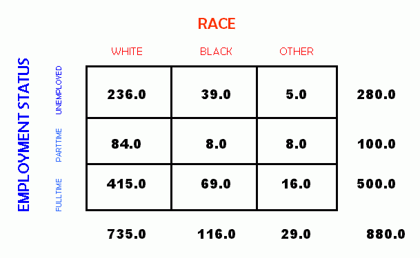
In this revised example, with one ordered variable and one categorical variable, we can continue to perform Chi-square calculations. However, since we have created an ordered variable, it is now possible to compare the means of the separate populations defined by the categorical variable, race. We can now use the ANOVA test to determine if there is a statistically significant difference in the means of the categories.
As a final example, consider what happens if we further collapse our example to divide race between "white" and "non-white". (For the purpose of what follows, we could equally well have used any category for the distinction.) The resulting crosstabulation is shown below.
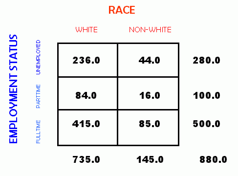
In this form of the example, we can (somewhat arbitrarily) assign numeric values of 0 to white and 1 to non-white. We can also assign numeric values to the levels of employment of 0 for unemployed, 1 for parttime employed, and 2 for fulltime employed. Once these scores are assigned, we can easily calculate Pearson's r for the example. Anytime that we can perform calculations on ordered rather than categorical variables, we can hope to obtain more information about existing relationships. For example, Chi-square can tell us if there is a statistically significant relationship hiding in data about salary versus educational level, but it does not tell us anything more than that certain cells in the crosstabulation have a value that is significantly different from the expected value. On the other hand, Pearson's r can tell us whether increased education leads to higher salary.
In this section we describe how to control for a third variable. The concept of "control" in statistics means to take into account the possible effect of a third variable on the relationship between the other two variables. We can observe the effects of the third variable on Chi-square by creating a separate crosstabulation table for each category of the third variable. For example, if we want to control for the effect of sex on the relationship between race and employment, we can make two separate crosstabulation tables, one for males and one for females.
Assuming that there is a relationship between race and employment, the question now is whether this relationship is affected by sex. If sex has no effect on the relationship, then the relationship holds (and is equally strong) regardless of the sex of the individual. On the other hand, if sex does have an effect on the relationship, then the strength of the relationship (and possibly even the existence of the relationship) will change depending on whether we look at males or females.
Consider what happens when we take a crosstabulation table (call it X), and double all of the cell values (and thus the marginals and grand total are doubled as well). Call this double-size table X2. The value for Chi-square in X2 is double that in X. Assume that the number of males and females in the population are equal. If we split table X2 into two to control for sex, we now have two tables of the same size as table X. If sex has no effect on the relationship between the variables, then the values for Chi-square are about equal to each other, and are about half the value of Chi-square for the combined table for both sexes.
On the other hand, if sex does effect the relationship between the other two variables, then the values for Chi-square for the tables should be different.
Below, we have a table that compares employment levels in whites and non-whites. Now, push the "split" button below this table. The resulting two tables give us a "control" for gender. In other words, we can now divide the results of the people looked at in the first table by gender. When we control for gender, does the Chi-square value change?
Activity 6
Activity 7
In the example, the value calculated for Chi-square on the entire population is not significantly different from the results we would get if there were no relationship between the variables. However, when we control for sex, we find that, for this sample, there is a greater effect of race on employment level for females than for males. The result is that, while the departure for the expected values goes down for males, it goes up for females. The resulting p value of .033, or 3.3% probability of occuring by chance, is statistically significant.
Return to Table of Contents