The current tutorial demonstrates how Multiple Regression is used in Social Sciences research. It is assumed that you are familiar with the concepts of correlation, simple linear regression, and hypothesis testing. If you are not familiar with these topics, please see the tutorials that cover them. We will first present an example problem to provide an overview of when multiple regression might be used. Then, we will address the following topics:
To conduct the study, all current retail sales employees at existing stores take psychological tests designed to measure intelligence and extroversion. Also, past sales performance data is checked for each employee. In the end, there are three scores for each sales person:
|
|
|
|
|
|
|
|
|
|
|
|
|
|
|
|
|
|
|
|
|
|
|
|
|
|
|
|
|
|
|
|
|
|
|
|
|
|
|
|
|
|
|
|
|
|
|
|
|
|
|
|
|
|
|
|
|
|
|
|
|
|
|
|
|
|
|
|
|
|
|
|
|
|
|
|
|
|
|
|
|
|
|
|
|
|
|
|
|
|
|
|
|
|
|
|
|
|
|
|
|
|
|
|
|
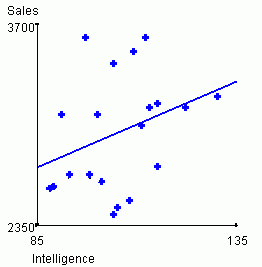
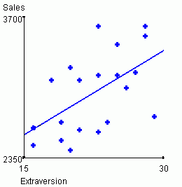
To analyze these data, one option is to examine the bivariate (i.e.,
two variable) correlation and the bivariate regression equation of the
intelligence vs. sales performance relationship and the extroversion vs.
sales performance relationship. For intelligence vs. sales performance,
the bivariate correlation r = .33 for the above data.
For the extroversion vs. sales relationship, r = .55.
Both of these relationships are positive, and are moderately strong relative to what is often observed
in "real world" studies similar to this. The interpretation is that
sales performance increases as ABC sales people become more intelligent
and more extroverted. The scatterplots and associated bivariate regression
equations shown below are another way to examine these data.
 |
 |
| Predicted sales = 1756.93 + 11.62*Intelligence | Predicted sales = 1759.67 + 54.12*Extraversion |
Although the bivariate analyses provide a perspective on how well each predictor forecasts sales performance, bivariate analyses cannot show how well the two predictors work together in predicting sales performance.
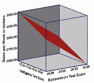
One way to assess how well the two predictors work together is to plot the data on a 3-dimensional graph. The graph below shows the relationship by graphing each salesperson's score. The intelligence score is plotted on the x-axis, the extroversion score is plotted on the z-axis, and sales performance is plotted on the y-axis.
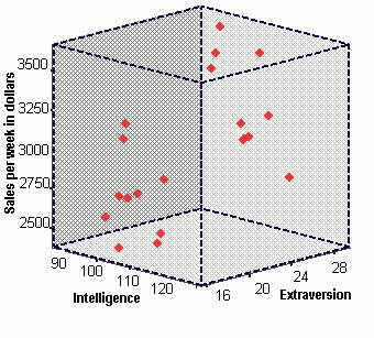
You probably can't infer much from the above plot. To aide in
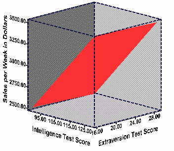
understanding the relationship, we present two copies of this plot below.
In the plots below, the observed data points have been removed, in order
for clarity of presentation. Both plots reflect the same data, but the
plots have been "rotated" so that you can view them from two different
angles. Further, the "regression plane" has been added to each plot in
the figures below. The regression plane is similar to the line of
best fit in simple bivariate regression, but now a plane is used instead
of a line because 3-dimensional data are used. This
regression plane summarizes the relationship between the three variables
such that the total distance between the points on the graph and the plane
are minimized--or what is known as the plane of best fit. The graphs
below show the plane of best fit for the ABC sales data above.
 |
 |
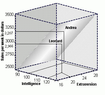
To predict sales performance for a potential new employee, you need that person's intelligence and extroversion scores. Then, all that you need to do is find the sales performance value that corresponds to the point on the regression plane for the applicant's intelligence and extroversion score. In the graph below, data for two hypothetical employees, Andrea and Leonard, are displayed along with the regression plane. Andrea has an Extroversion score of 28, and an Intelligence test score of 100. By graphing her Extroversion score and her Intelligence score, we can then plot her predicted weekly sales amount, which in this case is $3,207.00. Leonard, on the other hand, had an Intelligence test score of 119, and an Extroversion test score of 20. His predicted weekly sales would be $2,966.00.
Researchers commonly use regression equations to represent the relationships among predictor and criterion variables. This is true in both simple regression as well as multiple regression. The regression equation for the above data is:
Predicted sales performance = 993.93 + 8.22*Intelligence + 49.71*Extraversion
The first term in the prediction equation (993.93) is a constant that represents the predicted criterion value when both predictors equal zero. The values of 8.22 and 49.71 represent regression weights or regression coefficients. Multiplying an individual's intelligence score and extroversion score by the appropriate regression coefficient gives the predictor variable the statistically determined proper amount of weighting in predicting the criterion.
Once the mathematical formula for the regression equation is derived,
then it is a simple manner to predict sales performance of new applicants.
Each applicant is given an intelligence test and an extroversion test when
he/she applies for the job. The scores for the applicant are substituted
into the equation and then the equation is solved. The table below
gives some scores for three hypothetical applicants for the job.
On the basis of their intelligence test scores and their extroversion scores,
we can substitute these values into the equation and determine their predicted
weekly sales levels.
|
|
|
|
|
|
|
|
|||
| Steve J. |
|
|
|
|
|
|
|
|
|
| Erin N. |
|
|
|
|
|
|
|
|
|
| Chris B. |
|
|
|
|
|
|
|
|
|
If only one of these three applicants were to be hired, then based on this analysis, Erin N.
should be hired because she is predicted to have the highest amount of weekly
sales.
In the above exercise, you can explore the 3-dimensional scatterplot in a number of ways. First, use the pull down menu below the "criterion" heading to change the dependent variable. You will notice that the regression equation changes depending on which variable serves as the dependent variable. Now, change some of the actual data points in the table itself (make sure the values you select are in the range of 1 to 10). After you make any changes, simply click the update button or hit the "Enter" key to see how the 3-dimensional scatterplot changes. Also, be sure to notice how the regression equation changes as a function of the changes you make.
From the above information, you should have learned the following points:
- Researchers often predict a criterion using two or more predictors
- Researchers use multiple regression analysis to develop prediction models of the criterion
- In a graphic sense, multiple regression analysis models a "plane of best fit" through a scatterplot on the data.
- As the data points change in the scatterplot, the plane of best fit will change and the terms in the multiple regression equation will change.

The variables in the equation are  (the variable being predicted) and x1, x2, ..., xn
(the predictor variables in the equations). The "n" in xn
indicates that the number of predictors included is up to the researcher
conducting the study. It is not unusual for a researcher to use 4 or
5 predictors because generally speaking, the more predictors you have, the more accurately
the criterion will be predicted. In the equation, "a" is the y-intercept
which indicates the point at which the regression plane intersects the
y-axis when the values of the predictor scores are all zero.
The terms b1, b2, and bn are
all regression coefficients which are used as multipliers for the corresponding
predictor variables (i.e., x1, x2,and xn).
The computation for the regression coefficient in multiple regression analysis
is much more complex than in simple regression. In simple regression,
the regression weight includes information about the correlation between
the predictor and criterion plus information about the variability of both
the predictor and criteria. In multiple regression analysis, the
regression weight includes all this information, however, it also includes
information about the relationships between the predictor and all other
predictors in the equation and information about the relationship between
the criterion and all other predictors in the equation.
We will not burden you with the complex equation for computing a multiple regression coefficient. Instead we will focus on why all the added information about other predictors is included in the computation of the regression coefficient. In multiple regression, its quite common that two predictor variables capture some of the same variability in the criterion variable. That is, some of the variance that the first predictor explains in the criterion is the same variability that is explained by the second predictor variable. The more that two predictor variables are correlated with each other, the more likely it is that they capture the same variability in the criterion variable. In fact, if two predictor variables are perfectly correlated, then the variance that the first predictor explains in the criterion is exactly the same variability that the second predictor variable explains. In other words, the addition of the second predictor does not increase the ability to accurately forecast the criterion beyond what is accomplished by the first predictor.
A visual way to conceptualize this problem is through Venn diagrams. Each circle in the graph below represents the variance for each variable in a multiple regression problem with two predictors. When the two circles don't overlap, as they appear now, then none of the variables are correlated because they do not share variance with each other. In this situation, the regression weights will be zero because the predictors do not capture variance in the criterion variables (i.e., the predictors are not correlated with the criterion). This fact is summarized by a statistic known as the squared multiple correlation coefficient (R2). R2 indicates what percent of the variance in the criterion is captured by the predictors. The more criterion variance that is captured, the greater the researcher's ability to accurately forecast the criterion. In the exercise below, the circle representing the criterion can be dragged up and down. The predictors can be dragged left to right. At the bottom of the exercise, R2 is reported along with the correlations among the three variables. Move the circles back and forth so that they overlap to varying degrees. Pay attention to how the correlations change and especially how R2 changes. When the overlap between a predictor and the criterion is green, then this reflects the "unique variance" in the criterion that is captured by one predictor. However, when the two predictors overlap in the criterion space, you see red, which reflects "common variance". Common variance is a term that is used when two predictors capture the same variance in the criterion. When the two predictors are perfectly correlated, then neither predictor adds any predictive value to the other predictor, and the computation of R2 is meaningless.
To review, multiple regression coefficients are computed in such a way so that they not only take into account the relationship between a given predictor and the criterion, but also the relationships with other predictors. For this reason, researchers using multiple regression for predictive research strive to include predictors that correlate highly with the criterion, but that do not correlate highly with each other (i.e., researchers try to maximize unique variance for each predictors). To see this visually, go back to the Venn diagram above and drag the criterion circle all the way down, then drag the predictor circles so that they just barely touch each other in the middle of the criterion circle. When you achieve this, the numbers at the bottom will indicate that both predictors correlate with the criterion but the two predictors do not correlate with each other, and most importantly the R2 is large which means the criterion can be predicted with a high degree of accuracy.
Total Criterion Variability = Regression Effect + Residual Variation
This is an important formula for many reasons, but it is especially important because it is the foundation for statistical significance testing in multiple regression. Using simple regression (i.e., one criterion and one predictor), it will now be shown how to compute the terms of this equation.
Total Criterion Variability or SStotal = 
where Y is the observed score on the criterion,  is the criterion mean, and the S means to add
all these squared deviation scores together. Note that this value is not the variance in the criterion, but rather is
the sum of the squared deviations of all observed criterion scores from the mean value for the criterion.
Regression Effect or SSreg = 
where  is the predicted Y score
for each observed value of the predictor variable. That is,
  is the point on the line of best fit that corresponds to each observed
value of the predictor variable.
Residual Variance or SSres = 
That is, residual variance is the sum of the squared deviations between the observed criterion score and the corresponding predicted criterion score (for each observed value of the predictor variable).
Putting this all together, the formula for partitioning variance is:
 =
=  +
+ 
The above formula is much easier to understand graphically. Below is an exercise where you create a bivariate scatterplot. As you add, move, or delete points, you will notice that a regression line will be fit through the data. At the left-hand bottom you will see the regression equation (i.e., y = a + bx) and at the right-hand bottom you will see an equation of the partitioned variance for your scatterplot. You can view this scatterplot in two modes. In the "view SSreg mode", the scatterplot shows the deviations used to compute the SSreg. In the "view SSres mode", the scatterplot shows the deviations used to compute SSres. In this exercise, move the data points around so that you see a situation where the slope of the regression line is angled in relation to the regression line and then move the data points so that the slope of the regression line is parallel to the x-axis. Also, examine a scatterplot where the points cluster closely around the regression line and then move the points so that the points are scattered far from the regression line. In each situation, examine the regression equation and partitioned variance equation closely. See if you can discover the systematic relationship between the different scatterplots and the terms in the equations.
Hopefully, the above exercise allowed you to learn the following relationships:
Although the relationship between SSreg and SSres were demonstrated with bivariate regression examples, the logic holds true for multiple regression. SSreg and SSres can be computed for multiple regression analyses and researchers also prefer to see large SSreg and small SSres when using multiple regression.
More technically, when using either simple regression or multiple regression analyses for prediction, the researcher must decide if SSreg is large enough relative to SSres so as to be confident about using the regression equation to predict scores on the criterion. To aide this decision, researchers often use statistical significance testing to guide them. Formally stated, the researcher tests the null hypothesis that SSreg is equal to zero, against the alternative hypothesis that SSreg is greater than zero:
As seen in other tutorials, a statistical significance test of these hypotheses requires a sampling distribution. Statisticians have shown that the sampling distribution for the ratio of the regression effect (adjusted for degrees of freedom) to the residual variation (adjusted for degrees of freedom) is an F-distribution (See Analysis of Variance tutorial for the development of the F-distribution).
Using the ABC corporation data from above, the table below shows the "source table" for the simple regression analysis of the relationship between intelligence and sales performance. "Source table" is a generic term for a table that shows all the components necessary for computing F tests.
| Source | Sum of Squares | Degrees of Freedom | Mean Square | F | p |
|---|---|---|---|---|---|
| Regression | 314338.95 | 1 | 314338.95 | 2.19 | .16 |
| Residual | 2581411.00 | 18 | 143411.73 | ||
| Total | 2895750.00 | 19 |
The "Sum of Squares" terms reflect how the total variance in the criterion (i.e., sales performance) is partitioned by the regression effect due to intelligence and residual. To compute the F-ratio, the sum of squares regression and sum of squares residual are divided by their respective degrees of freedom, resulting in the mean square values. The F-ratio is computed by dividing the Mean Square Regression by the Mean Square Residual. The resulting F-ratio is compared to an F-table of critical values to see if the observed F-ratio is greater than would be expected on the basis of chance. Although not shown above, the critical value of the F-ratio with (1, 18) degrees of freedom and an alpha level of .05, is 4.41. The F-ratio observed in the table here is 2.19, which obviously is not greater than the critical value of 4.41. The "p" column in the above table also reflects the fact that our observed F-ratio is less than the F critical value (because .16 is > .05). Therefore the conclusion in this analysis is that the regression effect for intelligence is not greater than zero and thus intelligence alone may not be a good predictor of sales performance.
Below is the multiple regression source table for the ABC data using
both Intelligence and Extroversion to predict Sales Performance:
| Source | Sum of Squares | Degrees of Freedom | Mean Square | F | p |
|---|---|---|---|---|---|
| Regression | 1021166.40 | 2 | 510583.19 | 4.63 | .03 |
| Residual | 1874583.60 | 17 | 110269.63 | ||
| Total | 2895750.00 | 19 |
Although many of the values in the table have changed with the inclusion of extroversion, the computations needed for the F-ratio are the same. The critical value of the F-ratio with (2, 17) degrees of freedom at alpha = .05 is 3.59. The summary table above indicates that the regression effect is statistically significant because the observed F-ratio is greater than the critical value for F, and therefore the "p-value" for the regression effect is less than .05. In this case, the researcher concludes that the regression effect is greater than zero and that at least one of the predictors accurately forecast sales performance.
Now let's take a look at significance testing in the context of our earlier example where a researcher has measured Verbal Aptitude, Reading Ability, and Subject Motivation. As initially presented, the 3-D scatterplot at the top left represents the graphic representation of the data, the plane of best fit in the 3-D scatterplot is mathematically represented by the regression formula in the middle, the source table at the bottom indicates how the variance is partitioned between the regression effect and the residual variance, the F-ratio in the source table is essentially the proportion of the regression effect to the residual variation, and finally, the F-Distribution shows the relationship between the F-critical score (marked by a black line) and the observed F-value (marked with a red line). As shown, the regression effect for aptitude and motivation is significant. Therefore at least one of these predictors accurately forecast reading ability. Now change the criterion to motivation by selecting Motivation in the pull down menu under "criterion". This will automatically make verbal ability and reading ability predictors of motivation. How well do verbal ability and reading comprehension predict student motivation? There are a number of pieces of information that you can look at to answer this question. First, you can look at the three-dimensional scatterplot. Does there appear to be a linear relationship between the variables, or is the regression plane relatively flat? How about the observed F-ratio (as indicated by the red line in the graph)? Does it exceed the critical F-value (as indicated by the black line in the graph)? How about the regression coefficients for verbal ability and reading? Are they substantially larger than zero (i.e., greater than .30)?
If you changed the criterion to motivation, you saw that the regression effect was not significant. The observed F-value was 1.5685 which was much lower than the F-critical value. As such, you would fail to reject the null hypothesis that the regression effect is greater than zero and you would conclude that verbal ability and reading ability are not good predictors of motivation.
When testing the regression effect for significance in multiple regression
analysis, a significant effect simply indicates that at least one of the
predictors accurately forecasts the criterion to an extent which is greater than chance. Of course, a researcher
always wants to know exactly which predictor(s) are the source(s) of the
accurate forecasts. To determine which predictors are important in
the regression equation the researcher tests each regression coefficient
for significance.
H0: b1 = 0 and H0: ryx = 0
Remember that simple regression only has one predictor, which means that there is only one correlation (ryx ) being examined. That correlation is reflected in both the regression weight (b1) and SSreg. So if any one of the three is statistically significant, so are the other two. Technically speaking, researchers use a t-test to test the significance of simple regression weights and correlations because the t-test is a two-tailed significance test that allows researcher to test for values less then zero. That is, correlations and regression weights can be negative, therefore the two-tailed t-sampling distribution is needed. Whereas, SSreg can only be greater than zero (because the deviations are squared) which requires the one-tailed F-sampling distribution. Regardless of which sampling distribution is used, if one of these three (i.e., SSreg, b1, or ryx ) are determined to be statistically significant at a given level of alpha (or, at a given p value), then the other two are also statistically significant at that given level of alpha.
It's not so simple for multiple regression analysis. Because there are multiple predictors being used, a statistically significant SSreg only indicates that at least one of the predictors is significantly related to the criterion. Of course researchers want to know which predictors are producing the significant SSreg, so they automatically test each regression weight (i.e., b1, b2, to bn) for statistical significance. The formal hypotheses for this test are
H0: bn = 0
H1: bn  0
0
The use of bn is used to indicate that each predictor is tested separately from each other predictor. The computation of the t-value is simply

where sb is the standard error of the regression weight. The
computation for sb is statistically complex so it will not be presented here.
Each regression weight has it's own standard error estimate, so there are
as many standard errors of the regression weights as there are predictors.
This t-value is computed for each regression weight. The significance
of each predictor is determined by whether or not the observed t-value
for a predictor exceeds the critical t-value for the given level of alpha
being used. We evaluate the distribution of t for N - k - 1 degrees of freedom,
where k is equal to the total number of predictors in the regression equation. For the current analyses, the critical t-value
for the two-tailed tests of the significance of the regression coefficients for extroversion and intelligence is 1.74.
Below are the statistical significance tests for the regression weights in the ABC corporation example.
|
|
|
|
|
|
|
|
|
|
|
|
|
|
|
|
|
|
|
|
|
The t-value for the intelligence predictor does not exceed the t-critical value at .05, therefore, we fail to reject the null hypothesis that the intelligence regression coefficient is different than zero. However, the t-value for extroversion exceeds the t-critical value at .05, therefore, we reject that null hypothesis that the regression coefficient for extroversion is equal to zero. Although both extroversion and intelligence are positively related to sales performance, only extroversion is significantly related to sales performance. In plain terms, we are saying that only extroversion is an accurate predictor of sales performance, and as such, extroversion should be the only predictor of sales performance used by the ABC corporation. Although using an intelligence test might add some predictive value, it would not provide a significant level of predictive value, and as such, it would probably not be worth the time and expense for ABC Corporation to use intelligence tests when hiring employees.
It is critical to realize that in a standard (often called "simultaneous") multiple regression analysis the regression weight reflects only the "unique variance" attributable to each predictor. Remember that unique variance represents that percentage of the variance in the criterion that is captured only by one predictor. That is, the green area in the Venn diagram exercise above. As such common variance (i.e., the red area in the Venn diagram exercise above) does not contribute to the significance testing of individual regression coefficients when using simultaneous multiple regression.
The implication of each regression coefficient representing only unique variance captured by the predictor leads to different possibilities in terms of the results of statistical significance tests. The following patterns are all possible in a multiple regression analysis with two predictors:
| The image to the right illustrates this possibility. The circle at the top represents the variance in the criterion, and the circles below represent the variance in two different, but related, predictors. These predictors overlap with the criterion, and it is likely that the SSreg would be statistically significant when the criterion is regressed on the two predictors in a multiple regression analysis. However, most of the variance accounted for by these two predictors is common variance (that area indicated in red). When the regression coefficient for each of these predictors is tested for statistical significance, the analysis will be based on the unique variance accounted for by each predictor (the areas represented in green). It is likely that the tests of the regression coefficients associated with each of these predictors will not be statistically significant. When this happens, researchers will often eliminate one of the two predictors, since they overlap to such a degree. | 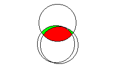 |
This scenario represents one important reason for using multiple regression. If the researcher had examined each of these two predictors independently, through the use of simple linear regression or bivariate correlations, she or he would probably have concluded that each was significantly related to the outcome variable. Through the use of multiple regression, we were able to discover that the two variables are in fact explaining redundant (common) variance in the outcome variable, and we can eliminate one without losing much predictive power.
Return to Table of Contents