Range

1. As a quantity: the difference between the highest and lowest scores in a distribution.
   "The range of scores on the exam was 32."
2. As an interval; the lowest and highest scores may be reported as the range.
   "The range was 62 to 94," which would be written (62, 94).

NUMBER OF BROTHERS AND SISTERS { 2, 3, 1, 1, 0, 5, 3, 1, 2, 7, 4, 0, 2, 1, 2, 1, 6, 3, 2, 0, 0, 7, 4, 2, 1, 1, 2, 1, 3, 5, 12, 4, 2, 0, 5, 3, 0, 2, 2, 1, 1, 8, 2, 1, 2 }

Percentiles and related characteristics

Percentile describes the relative location of points anywhere along the range of a distribution. A score that is at a certain percentile falls even with or above that percent of scores. The median score of a distribution is at the 50th percentile: It is the score at which 50% of other scores are below (or equal) and 50% are above. Commonly used percentile measures are named in terms of how they divide distributions. Quartiles divide scores into fourths, so that a score falling in the first quartile lies within the lowest 25% of scores, while a score in the fourth quartile is higher than at least 75% of the scores.

The divisions you have just performed illustrate quartile scores. Two other percentile scores commonly used to describe the dispersion in a distribution are decile and quintile scores which divide cases into equal sized subsets of tenths (10%) and fifths (20%), respectively. In theory, percentile scores divide a distribution into 100 equal sized groups. In practice this may not be possible because the number of cases may be under 100.

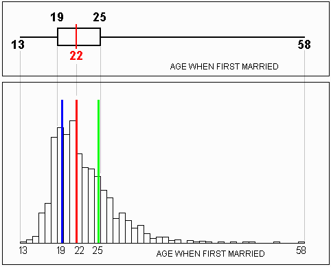
A box plot is an effective visual representation of both central tendency and dispersion. It simultaneously shows the 25th, 50th (median), and 75th percentile scores, along with the minimum and maximum scores. The "box" of the box plot shows the middle or "most typical" 50% of the values, while the "whiskers" of the box plot show the more extreme values. The length of the whiskers indicate visually how extreme the outliers are.

Below is the box plot for the distribution you just separated into quartiles. The boundaries of the box plot's "box" line up with the columns for the quartile scores on the histogram. The box plot displays the median score and shows the range of the distribution as well.

Variance and Standard Deviation

In calculating the variance of data points, we square the difference between each point and the mean because if we summed the differences directly, the result would always be zero. For example, suppose three friends work on campus and earn $5.50, $7.50, and $8 per hour, respectively. The mean of these values is $(5.50 + 7.50 + 8)/3 = $7 per hour. If we summed the differences of the mean from each wage, we would get (5.50-7) + (7.50-7) + (8-7) = -1.50 + .50 + 1 = 0. Instead, we square the terms to obtain a variance equal to 2.25 + .25 + 1 = 3.50. This figure is a measure of dispersion in the set of scores.

The variance is the minimum sum of squared differences of each score from any number. In other words, if we used any number other than the mean as the value from which each score is subtracted, the resulting sum of squared differences would be greater. (You can try it yourself -- see if any number other than 7 can be plugged into the preceeding calculation and yield a sum of squared differences less than 3.50.)

The standard deviation is simply the square root of the variance. In some sense, taking the square root of the variance "undoes" the squaring of the differences that we did when we calculated the variance.

Variance and standard deviation of a population are designated by  and  , respectively. Variance and standard deviation of a sample are designated by s² and s, respectively.

	Variance	Standard Deviation
Population
Sample

In these equations,   is the population mean,   is the sample mean, N is the total number of scores in the population, and n is the number of scores in the sample.

Comparisons of Measures of Dispersion

Range. Of all the measures of dispersion, the range is the easiest to determine. It is commonly used as a preliminary indicator of dispersion. However, because it takes into account only the scores that lie at the two extremes, it is of limited use.

Quartile Scores are based on more information than the range and, unlike the range, are not affected by outliers. However, they are only infrequently used to describe dispersion because they are not as easy to calculate as the range and they do not have the mathematical properties that make them so useful as standard deviation and variance.

The standard deviation ( or s) and variance ( or s²) are more complete measures of dispersion which take into account every score in a distribution. The other measures of dispersion we have discussed are based on considerably less information. However, because variance relies on the squared differences of scores from the mean, a single outlier has greater impact on the size of the variance than does a single score near the mean. Some statisticians view this property as a shortcoming of variance as a measure of dispersion, especially when there is reason to doubt the reliability of some of the extreme scores. For example, a researcher might believe that a person who reports watching television an average of 24 hours per day may have misunderstood the question. Just one such extreme score might result in an appreciably larger standard deviation, especially if the sample is small. Fortunately, since all scores are used in the calculation of variance, the many non-extreme scores (those closer to the mean) will tend to offset the misleading impact of any extreme scores.

The standard deviation and variance are the most commonly used measures of dispersion in the social sciences because:

• Both take into account the precise difference between each score and the mean. Consequently, these measures are based on a maximum amount of information.
• The standard deviation is the baseline for defining the concept of standardized score or "z-score".
• Variance in a set of scores on some dependent variable is a baseline for measuring the correlation between two or more variables (the degree to which they are related).

Standardized Distribution Scores, or "Z-Scores"

When we are given an absolute deviation from the mean, expressed in terms of empirical units, it is difficult to tell if the difference is "large" or "small" compared to other members of the data set. In the above example, are there many families that make less money than the Smith family, or only a few? We were not given enough information to decide.

We get more information about deviation from the mean when we use the standard deviation measure presented earlier in this tutorial. Raw scores expressed in empirical units can be converted to "standardized" scores, called z-scores. The z-score is a measure of how many units of standard deviation the raw score is from the mean. Thus, the z-score is a relative measure instead of an absolute measure. This is because every individual in the dataset affects value for the standard deviation. Raw scores are converted to standardized z-scores by the following equations:

Population z-score
Sample z-score

where  is the population mean,   is the sample mean,   is the population standard deviation, s is the sample standard deviation, and x is the raw score being converted.

For example, if the mean of a sample of I.Q. scores is 100 and the standard deviation is 15, then an I.Q. of 128 would correspond to:

= (128 - 100) / 15 = 1.87

z = (90 - 100) / 15 = - 0.67

Z-scores allow for control across different units of measure. For example, an income that is 25,000 units above the mean might sound very high for someone accustomed to thinking in terms of U.S. dollars, but if the unit is much smaller (such as Italian Lires or Greek Drachmas), the raw score might be only slightly above average.  Z-scores provide a standardized description of departures from the mean that control for differences in size of empirical units.

When a dataset conforms to a "normal" distribution, each z-score corresponds exactly to known, specific percentile score. If a researcher can assume that a given empirical distribution approximates the normal distribution, then he or she can assume that the data's z-scores approximate the z-scores of the normal distribution as well. In this case, z-scores can map the raw scores to their percentile scores in the data.

As an example, suppose the mean of a set of incomes is $60,200, the standard deviation is $5,500, and the distribution of the data values approximates the normal distribution. Then an income of $69,275 is calculated to have a z-score of 1.65. For a normal distribution, a z-score of 1.65 always corresponds to the 95th percentile. Thus, we can assume that $69,275 is the 95th percentile score in the empirical data, meaning that 95% of the scores lie at or below $69,275.

The normal distribution is a precisly defined, theoretical distribution. Empirical distributions are not likely to conform perfectly to the normal distribution. If the data distribution is unlike the normal distribution, then z-scores do not translate to percentiles in the "normal" way. However, to the extent that an empirical distribution approximates the normal distribution, z-scores do translate to percentiles in a reliable way.
 

Summary

• Range,
• Percentile Scores, and particularly, Quartile Scores,
• Variance,
• Standard Deviation,
• Z-Scores as a means of locating approximate percentile scores.

It it interesting to note that two sets of data might each have the same mean value, but very different dispersions. Likewise, two data sets might have similar ranges, or similar standard deviations, while having different means.

Return to Table of Contents